3 Part 2 - Analyzing Data

3.1 Intended Learning Outcomes

Be introduced to key dplyr functions for data wrangling (part of the tidyverse)
Be able to create numerical summaries of data
Be able to create graphical summaries of data
Be able to create objects by writing and running code in the console

3.2 Dealing with Data: Great British Bake Off (GBBO)

The data set we will be looking at in this section refers to TV competition "Great British Bake Off" (often abbreviated to "Bake Off" or "GBBO"). Within each series, a group of amateur bakers compete against each other in a series of episodes, attempting to impress a group of judges with their baking skills. One contestant is eliminated in each episode, and the winner is selected from the contestants who reach the final. The first episode was aired on 17 August 2010, with its first four series broadcast on BBC Two, after which it moved to BBC One for the next three series. After its seventh series, it moved to Channel 4.

3.2.1 Reading data in

The text file ratings_seasons.csv contains data on the first 10 series (2010-2019) of GBBO which can be imported using the following code.

ratings <- read.csv(url("https://raw.githubusercontent.com/craigalexander/AdvHStatsLab2/main/ratings_seasons.csv"))

3.2.2 Looking at data

Now that you've loaded some data, look the upper right hand window of RStudio, under the Environment tab. You will see the object ratings listed, along with the number of observations (rows) and variables (columns). This is your first check that you've read in the data correctly.

Always look at your data once you've created or loaded it. Also look at it after each step that transforms your data. There are two main ways to look at your data: View() and str().

View()

An intuitive way to look at the data is by using View() (uppercase 'V'), which opens up a data table in the console pane using a viewer that looks a bit like an Excel spreadsheet. This command can be useful in the console, but don't ever put this one in a script because it will create an annoying pop-up window when the user runs it. You can also click on an object in the Environment pane to open it in the same interface. You can close the tab when you're done looking at it; it won't remove the object containing the data.

View(ratings)

str()

The funciton str() (short for "structure") shows the number of observations and variables and the datatype of those variables, e.g. "num" for an number, "chr" for a character string (and a lot more information that we don't need to know about!)

str(ratings, give.attr=FALSE)  #The argument give.attr=FALSE surpresses extra info

## 'data.frame':    94 obs. of  11 variables:
##  $ series              : int  1 1 1 1 1 1 2 2 2 2 ...
##  $ episode             : int  1 2 3 4 5 6 1 2 3 4 ...
##  $ uk_airdate          : chr  "2010-08-17" "2010-08-24" "2010-08-31" "2010-09-07" ...
##  $ viewers_7day        : num  2.24 3 3 2.6 3.03 2.75 3.1 3.53 3.82 3.6 ...
##  $ viewers_28day       : num  7 3 2 4 1 1 2 2 1 1 ...
##  $ network_rank        : int  NA NA NA NA NA NA NA NA NA NA ...
##  $ channels_rank       : int  NA NA NA NA NA NA NA NA NA NA ...
##  $ bbc_iplayer_requests: int  NA NA NA NA NA NA NA NA NA NA ...
##  $ episode_count       : int  1 2 3 4 5 6 7 8 9 10 ...
##  $ us_season           : int  NA NA NA NA NA NA NA NA NA NA ...
##  $ us_airdate          : chr  NA NA NA NA ...

It is always necessary to look at the data you are working with to get a good sense of what it contains, i.e. the different types of data contained in the data set and how much data you have.

We used the str() function above to get information on the number of variables and observations and to list the variables together with the first few values they take.

Alternatively we could use these functions:

head(): shows the first 6 lines of the first few variables

head(ratings)

##   series episode uk_airdate viewers_7day viewers_28day network_rank
## 1      1       1 2010-08-17         2.24             7           NA
## 2      1       2 2010-08-24         3.00             3           NA
## 3      1       3 2010-08-31         3.00             2           NA
## 4      1       4 2010-09-07         2.60             4           NA
## 5      1       5 2010-09-14         3.03             1           NA
## 6      1       6 2010-09-21         2.75             1           NA
##   channels_rank bbc_iplayer_requests episode_count us_season us_airdate
## 1            NA                   NA             1        NA       <NA>
## 2            NA                   NA             2        NA       <NA>
## 3            NA                   NA             3        NA       <NA>
## 4            NA                   NA             4        NA       <NA>
## 5            NA                   NA             5        NA       <NA>
## 6            NA                   NA             6        NA       <NA>

glimpse(): gives a sideways version of the data. This is useful if the data is very wide (i.e. has lots of variables) and you can't easily see all of the columns/variables. It also tells you the data type of each column/variable in angled brackets after each column/variable name.

glimpse(ratings)

## Rows: 94
## Columns: 11
## $ series               <int> 1, 1, 1, 1, 1, 1, 2, 2, 2, 2, 2, 2, 2, 2, 3, 3, 3~
## $ episode              <int> 1, 2, 3, 4, 5, 6, 1, 2, 3, 4, 5, 6, 7, 8, 1, 2, 3~
## $ uk_airdate           <chr> "2010-08-17", "2010-08-24", "2010-08-31", "2010-0~
## $ viewers_7day         <dbl> 2.24, 3.00, 3.00, 2.60, 3.03, 2.75, 3.10, 3.53, 3~
## $ viewers_28day        <dbl> 7, 3, 2, 4, 1, 1, 2, 2, 1, 1, 1, 1, 1, 1, 1, 1, 1~
## $ network_rank         <int> NA, NA, NA, NA, NA, NA, NA, NA, NA, NA, NA, NA, N~
## $ channels_rank        <int> NA, NA, NA, NA, NA, NA, NA, NA, NA, NA, NA, NA, N~
## $ bbc_iplayer_requests <int> NA, NA, NA, NA, NA, NA, NA, NA, NA, NA, NA, NA, N~
## $ episode_count        <int> 1, 2, 3, 4, 5, 6, 7, 8, 9, 10, 11, 12, 13, 14, 15~
## $ us_season            <int> NA, NA, NA, NA, NA, NA, NA, NA, NA, NA, NA, NA, N~
## $ us_airdate           <chr> NA, NA, NA, NA, NA, NA, NA, NA, NA, NA, NA, NA, N~

By using any of the methods described above, answer these questions:

How many variables does the data ratings contain?
How many observations does ratings contain?

In this tutorial we are interested in the ratings of each episode in the 7 day period after its broadcast.

What variable contains this information?

3.2.3 Exploring data

The variables we will analyse in this tutorial are:

series: the series number, ranging from 1 to 10 corresponding to 2010-2019.
episode: the episode number, randing from 1 to 10 (although not all series had 10 episodes!)
viewers_7day the ratings of each episode in the 7 day period after its broadcast (measured as millions of viewers)

Run this code to just see the viewers_7day values in the ratings data:

ratings$viewers_7day

##  [1]  2.240  3.000  3.000  2.600  3.030  2.750  3.100  3.530  3.820  3.600
## [11]  3.830  4.250  4.420  5.060  3.850  4.600  4.530  4.710  4.610  4.820
## [21]  5.100  5.350  5.700  6.740  6.600  6.650  7.170  6.820  6.950  7.320
## [31]  7.760  7.410  7.410  9.450  8.510  8.790  9.280 10.250  9.950 10.130
## [41] 10.280  9.023 10.670 13.510 11.620 11.590 12.010 12.360 12.390 12.000
## [51] 12.350 11.090 12.650 15.050 13.580 13.450 13.010 13.290 13.120 13.130
## [61] 13.450 13.260 13.440 15.900  9.460  9.230  8.680  8.550  8.610  8.610
## [71]  9.010  8.950  9.030 10.040  9.550  9.310  8.910  8.880  8.670  8.910
## [81]  9.220  9.690  9.500 10.340  9.620  9.380  8.940  8.960  9.260  8.700
## [91]  8.980  9.190  9.340 10.050

What do the numbers in square brackets represent in the output to ratings$viewers_7day?

They are part of the data set, i.e. more values of ratings. They don't really have any important meaning. They represent the time taken to run the code in miliseconds. They represent the position of the ratings in the output. i.e. [1] preceeds the first ratings value, [21] preceeds the 21st ratings value.

3.3 `dplyr` functions for data wrangling

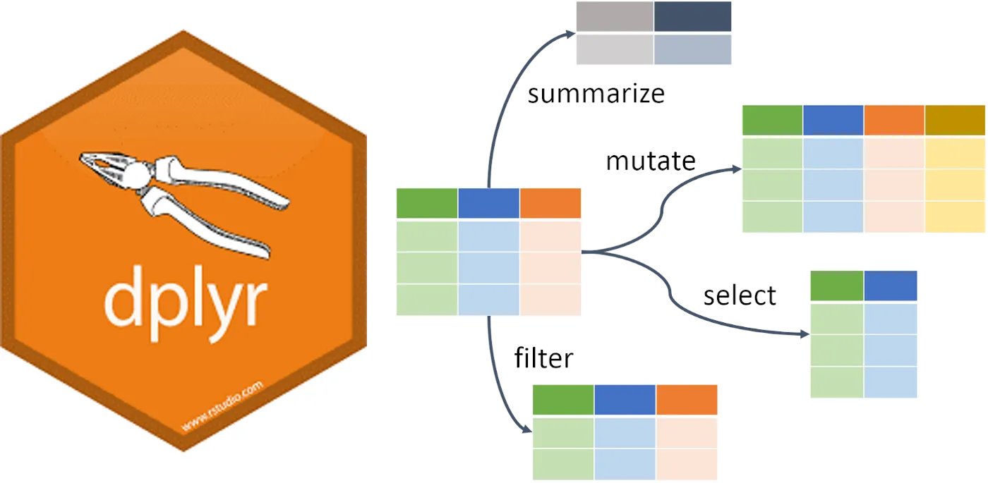
We're now going to use some key functions in the dplyr package (part of the tidyverse) to "wrangle" data.

If you haven't already, load the tidyverse package by copying and running this code in your script file:

library(tidyverse)

3.3.1 Creating a new variable and adding it to a data object

Not all the information we need is necessarily included in the data. For example, the viewers_7day variable is measured as millions of viewers, but what if we wanted it to be in raw numbers (i.e. 15000000 instead of 1.5)? Also, in the introduction to the GBBO data we were told the "first four series [were] broadcast on BBC Two, after which it moved to BBC One for the next three series. After its seventh series, it moved to Channel 4.". We can add this information to the ratings data as another variable/column in the ratings data.

Run this code to create a new variables viewers_7day_raw and channel in the ratings data and print it to check that it as we intended:

ratings <- mutate(ratings, 
                  viewers_7day_raw = viewers_7day * 1000000,
                  channel = case_when(series < 5 ~ "BBC2",
                                                series > 4 & series <8 ~ "BBC1",
                                                series > 7 ~ "C4"))

ratings$viewers_7day_raw
select(ratings, series, channel)

Before we proceed to creating summarisies of variables we need to pause and think about two types of variables: numeric and categorical.

**Run this code again to see the variables (including the one we've just added) in ratings

str(ratings)

## 'data.frame':    94 obs. of  13 variables:
##  $ series              : int  1 1 1 1 1 1 2 2 2 2 ...
##  $ episode             : int  1 2 3 4 5 6 1 2 3 4 ...
##  $ uk_airdate          : chr  "2010-08-17" "2010-08-24" "2010-08-31" "2010-09-07" ...
##  $ viewers_7day        : num  2.24 3 3 2.6 3.03 2.75 3.1 3.53 3.82 3.6 ...
##  $ viewers_28day       : num  7 3 2 4 1 1 2 2 1 1 ...
##  $ network_rank        : int  NA NA NA NA NA NA NA NA NA NA ...
##  $ channels_rank       : int  NA NA NA NA NA NA NA NA NA NA ...
##  $ bbc_iplayer_requests: int  NA NA NA NA NA NA NA NA NA NA ...
##  $ episode_count       : int  1 2 3 4 5 6 7 8 9 10 ...
##  $ us_season           : int  NA NA NA NA NA NA NA NA NA NA ...
##  $ us_airdate          : chr  NA NA NA NA ...
##  $ viewers_7day_raw    : num  2240000 3000000 3000000 2600000 3030000 2750000 3100000 3530000 3820000 3600000 ...
##  $ channel             : chr  "BBC2" "BBC2" "BBC2" "BBC2" ...

The values just after the ":" tells us the type of each variable

int stands for integer which is a numeric variable
chr stands for 'character' which usually represents a categorical variable

Because numbers (e.g. the values that series takes, i.e. 1, 2, 3, ...) can also represent 'categories' or 'levels' of a categorical variable, R doesn't assume that just because a variable is of type chr that it is categorical. To specify a categorical variable in R we use the as.factor() function, since R calls categorical variables "factors". In the ratings data the three variables series, episode and channel are categorical variables but they aren't stored as such, yet!

To tell R that variables are factors (i.e. categorical) use mutate() to overriding the original variable with the same data but classified as a factor.

Copy and run this code to change the series, episode and channel variables to factors.

ratings <- ratings %>%
  mutate(series = as.factor(series),
         episode = as.factor(episode),
         channel = as.factor(channel))
str(ratings)

## 'data.frame':    94 obs. of  13 variables:
##  $ series              : Factor w/ 10 levels "1","2","3","4",..: 1 1 1 1 1 1 2 2 2 2 ...
##  $ episode             : Factor w/ 10 levels "1","2","3","4",..: 1 2 3 4 5 6 1 2 3 4 ...
##  $ uk_airdate          : chr  "2010-08-17" "2010-08-24" "2010-08-31" "2010-09-07" ...
##  $ viewers_7day        : num  2.24 3 3 2.6 3.03 2.75 3.1 3.53 3.82 3.6 ...
##  $ viewers_28day       : num  7 3 2 4 1 1 2 2 1 1 ...
##  $ network_rank        : int  NA NA NA NA NA NA NA NA NA NA ...
##  $ channels_rank       : int  NA NA NA NA NA NA NA NA NA NA ...
##  $ bbc_iplayer_requests: int  NA NA NA NA NA NA NA NA NA NA ...
##  $ episode_count       : int  1 2 3 4 5 6 7 8 9 10 ...
##  $ us_season           : int  NA NA NA NA NA NA NA NA NA NA ...
##  $ us_airdate          : chr  NA NA NA NA ...
##  $ viewers_7day_raw    : num  2240000 3000000 3000000 2600000 3030000 2750000 3100000 3530000 3820000 3600000 ...
##  $ channel             : Factor w/ 3 levels "BBC1","BBC2",..: 2 2 2 2 2 2 2 2 2 2 ...

You can read this code as, for example, "overwrite the data that is in the column series with series as a factor, thus converting it to a categorical variable".

Remember this. It's a really important step and if graphs are looking weird this might be the reason.

3.3.2 Creating summaries of data

3.3.2.1 Numerical Data

The summarise() function from the dplyr package is loaded as part of the tidyverse and creates summary statistics. It creates a new object with columns that summarise the data from a larger table using summary functions. Check this Cheat Sheet for various summary functions. Some common ones are: n(), min(), max(), mean(), sd() and quantile().

Here is an example using summarise()

summarise(ratings,
      mean_ratings = mean(viewers_7day),
      sd_ratings = sd(viewers_7day),
      min_ratings = min(viewers_7day),
      max_ratings = max(viewers_7day))

##   mean_ratings sd_ratings min_ratings max_ratings
## 1     8.579606   3.266634        2.24        15.9

The first argument that summarise() takes is the data object to summarise
summarise() creates a new object. The column names of this new object are on the left hand-side of =, i.e., mean_ratings, sd_ratings, min_ratings and max_ratings.
The values of these columns are the result of the summary operation on the right hand-side of =.

What is the average number of viewers that GBBO had in the 7 days after broadcast?

3270000 2240000 8580000 15900000

What is the least number of viewers that GBBO had in the 7 days after broadcast:
What is the most viewers that GBBO had in the 7 days after broadcast:

3.3.2.2 Categorical Data

All of the summaries considered above are relevant for numercial/continuous variables but there also categorical variables in the ratings data.

Identify the type of each of the variables in the ratings data:

series:
episode:
viewers_7day
channel

The count() function counts the number of rows that are the same. This will give you a new table with each combination of the counted rows and a column called n containing the number of observations from that group.

The first argument that count() takes is the data object to summarise
The next arguments that count() takes are the variables to summarise
The argument sort = TRUE will sort the table by n in descending order.
Look at the output from this code and answer the following question:

  count(ratings, channel, sort = TRUE)

##   channel  n
## 1    BBC2 34
## 2    BBC1 30
## 3      C4 30

Which channel screened the most episodes of GBBO from 2010 to 2019?
Look at the output from this code and answer the following questions:

  count(ratings, channel, series)

##    channel series  n
## 1     BBC1      5 10
## 2     BBC1      6 10
## 3     BBC1      7 10
## 4     BBC2      1  6
## 5     BBC2      2  8
## 6     BBC2      3 10
## 7     BBC2      4 10
## 8       C4      8 10
## 9       C4      9 10
## 10      C4     10 10

What is this summary revealing?

The number of episodes within each series (together with what channel broadcast that series) The number of series within each episode (together with what channel broadcast that series) The number of series within each episode The number of episodes within each series

How could the order of the columns in the summary table be changed?

The order can't be changed count(ratings, series, episode) count(ratings, episode, channel) count(ratings, series, channel)

3.3.2.3 Summarising Numerical and Categorical Data Simultaneously

Its seldom that we are interested in just one variable at a time. An example of this is when we want numerical summaries but for each category/group of a categorical variable. The combination of the group_by() and summarise() functions is incredibly powerful for this task (and it is also a good demonstration of why pipes (%>%) are so useful!).

The function group_by() takes an existing data object and converts it into a grouped object, where any operations that are performed on it are done "by group".

Consider this code and its output:

ratings_grouped <- ratings %>%
  group_by(channel)

ch_ratings <- ratings_grouped %>%
  summarise(count = n(),
            mean_ratings = mean(viewers_7day),
            min_ratings = min(viewers_7day),
            max_ratings = max(viewers_7day)) %>%
  ungroup()

ch_ratings

## # A tibble: 3 x 5
##   channel count mean_ratings min_ratings max_ratings
##   <fct>   <int>        <dbl>       <dbl>       <dbl>
## 1 BBC1       30        12.0         8.51       15.9 
## 2 BBC2       34         5.05        2.24        9.45
## 3 C4         30         9.19        8.55       10.3

Make sure you call the ungroup() function when you are done with grouped functions. Failing to do this can cause all sorts of mysterious problems if you use that data object later assuming it isn't grouped.

The first line of code below creates an object named ratings_grouped, that groups the data according to what channel the episode was broadcast on.
On the surface, ratings_grouped doesn't look any different to the original ratings data.
However, the underlying structure has changed and so when we run summarise(), we now get our requested summaries for each group (in this case for each channel).

Whilst the above code is functional, it adds an unnecessary object to the environment - ratings_grouped is taking up space and increases the risk we'll use this grouped object by mistake. A better way to do this is to use the pipe (>%>.

Rather than creating an intermediate object, we can use the pipe to string our code together.

Run this code and check that the object produced is identical to ch_ratings shown above.

ch_ratings <- 
  ratings %>%             # Start with the original dataset; and then
  group_by(channel) %>%   # group it; and then
  summarise(count = n(),  # summarise it by those groups
            mean_ratings = mean(viewers_7day),
            min_ratings = min(viewers_7day),
            max_ratings = max(viewers_7day)) %>%
  ungroup()

What would you change to calculate the mean ratings by series instead of by channel?

group_by(series) summarise(series) count(series) mean(series)

You can add multiple variables to group_by() to further break down your data. For example, the below gives us the average ratings broken down by channel and series.

Reverse the order of channel and series in group_by() to see how it changes the output.

ch_series_ratings <- 
  ratings %>%             
  group_by(channel, series) %>%   
  summarise(count = n(),
            mean_ratings = mean(viewers_7day),
            min_ratings = min(viewers_7day),
            max_ratings = max(viewers_7day)) %>%
  ungroup()

ch_series_ratings

## # A tibble: 10 x 6
##    channel series count mean_ratings min_ratings max_ratings
##    <fct>   <fct>  <int>        <dbl>       <dbl>       <dbl>
##  1 BBC1    5         10        10.0         8.51       13.5 
##  2 BBC1    6         10        12.3        11.1        15.0 
##  3 BBC1    7         10        13.6        13.0        15.9 
##  4 BBC2    1          6         2.77        2.24        3.03
##  5 BBC2    2          8         3.95        3.1         5.06
##  6 BBC2    3         10         5.00        3.85        6.74
##  7 BBC2    4         10         7.35        6.6         9.45
##  8 C4      8         10         9.02        8.55       10.0 
##  9 C4      9         10         9.30        8.67       10.3 
## 10 C4      10        10         9.24        8.7        10.0

Which code lists the summaries in chronological order?